High-level analysis in FSL aggregates results from individual subjects to draw inferences about a population. The typical steps involve:
- Data collection: Gather first-level FEAT outputs (cope, varcope, and sometimes t-statistic images).
- Design specification: Define your design matrix and contrast vectors to model group-level effects.
- Estimation: Use FSL’s FEAT (or FLAME) for mixed-effects analysis.
- Inference: Correct for multiple comparisons and interpret cluster or voxel-level results.
1. Prepare your first-level data
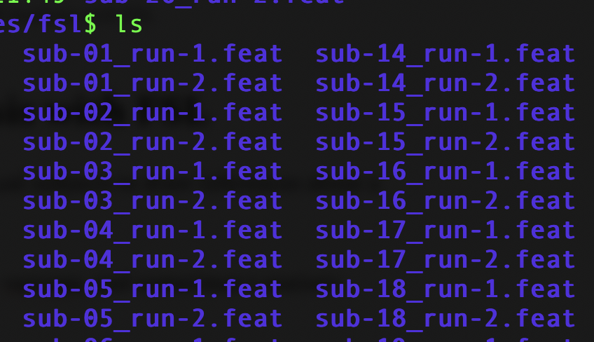
After the first-level analysis, you have the necessary data organized. For example, you put all subject-wise data in subfolder derivatives:
2. Create Design and Contrast Matrix
Open Feat & GUI, and add all first-level feat folders or COPE files, depending on your experimental design.
Andy Jahn’s brain book website provides excellent instructions on this. Please check his second-level analysis and third-level analysis for details.
Essentially, you need to create a higher-level analysis by setting up a new FEAT design file. Here is an example of such design file:
# Higher-level FEAT design example for one-sample t-test

# Set the basic parameters
# For higher-level analysis, npts = number of input cope files (i.e. subjects)
set fmri(npts) 3
set fmri(outputdir) "group_level.feat"

# Input subject-level cope images
set feat_files(1) "/path/to/sub01/first_level.feat/stats/cope1.nii.gz"
set feat_files(2) "/path/to/sub02/first_level.feat/stats/cope1.nii.gz"
set feat_files(3) "/path/to/sub03/first_level.feat/stats/cope1.nii.gz"
# ... add more subjects as needed

# Define the design matrix file paths
set fmri(groupfile) "feat_dir_list.txt"
set fmri(cope1) 1

# Set up the design for a one-sample t-test
set fmri(contrasts) "1"
set fmri(contrast_names1) "Mean Effect"

# Higher-level model — FSL's mixed_yn codes (note: NOT in ascending order):
#   3 = Fixed effects
#   0 = Mixed Effects: Simple OLS
#   2 = Mixed Effects: FLAME 1      <- the usual group-level choice
#   1 = Mixed Effects: FLAME 1+2
# FLAME 1 (value 2) refines variance estimation using each subject's lower-level
# variance; FLAME 1+2 (value 1) adds a slower second stage for marginal voxels.
set fmri(mixed_yn) 2
The above example uses FLAME 1 (FMRIB’s Local Analysis of Mixed Effects).
fixed effects vs OLS vs FLAME 1 vs FLAME 1+2
The FSL numeric codes are not in ascending order — copy them carefully.
- Fixed effects (
fmri(mixed_yn) 3) — ignores between-subject variance entirely; inference applies only to this sample, not the population. Appropriate for within-subject averaging (e.g. combining a subject’s runs), never for population-level group inference.- Mixed Effects: Simple OLS (
fmri(mixed_yn) 0) — models random effects but with a crude equal-variance estimate that ignores each subject’s lower-level variance. Fast; the least accurate mixed-effects option.- Mixed Effects: FLAME 1 (
fmri(mixed_yn) 2) — one Bayesian/MCMC pass per voxel, weighting subjects by their lower-level variance. The standard, well-validated choice for group inference. Use this by default.- Mixed Effects: FLAME 1+2 (
fmri(mixed_yn) 1) — adds a second, slower MCMC stage for voxels near threshold. Marginally tightens borderline voxels at large compute cost (~10× slower). Use only when reviewers demand it.
3. Worked example: 10-subject one-sample t-test
Below is a minimal end-to-end recipe for a group-level one-sample t-test on the first-level cope1 images of ten subjects. The goal is to test whether the contrast mean is non-zero across the group. We avoid the FEAT GUI here and drive flameo directly, which is the engine FEAT calls under the hood.
3.1 Set up environment
Use environment variables rather than hard-coded paths so the script ports between datasets and machines:
export FMRIPREP_DIR=/data/derivatives/fmriprep
export LEVEL1_DIR=/data/derivatives/level1
export LEVEL2_DIR=/data/derivatives/level2/onesample_cope1
mkdir -p "$LEVEL2_DIR"
cd "$LEVEL2_DIR"
3.2 Collect the first-level COPE images
A small bash glob loop collects all subject-level cope1 files and counts them. Sanity-check the count before proceeding:
copes=()
for f in ${LEVEL1_DIR}/sub-*/cope1.nii.gz; do
    [ -f "$f" ] || continue
    copes+=("$f")
done
N=${#copes[@]}
echo "Found $N cope images"
# Expect: Found 10 cope images
Do the same for the matching varcope1.nii.gz files — FLAME needs both:
varcopes=()
for f in ${LEVEL1_DIR}/sub-*/varcope1.nii.gz; do
    varcopes+=("$f")
done
3.3 Merge into 4D and build a group mask
flameo expects merged 4D inputs (one volume per subject) and a common mask. A conservative group mask is the intersection of the individual brain masks:
fslmerge -t merged_cope.nii.gz    "${copes[@]}"
fslmerge -t merged_varcope.nii.gz "${varcopes[@]}"

# Group mask = voxels present in every subject
fslmerge -t merged_mask.nii.gz ${LEVEL1_DIR}/sub-*/mask.nii.gz
fslmaths merged_mask.nii.gz -Tmin group_mask.nii.gz
3.4 Write the design files with Text2Vest
For a one-sample t-test the design is a column of ones, the contrast is a single 1, and every subject belongs to the same variance group. Text2Vest converts plain text into FSL’s VEST format:
# design.txt: N rows of "1"
yes 1 | head -n $N > design.txt
Text2Vest design.txt design.mat

# contrast.txt: single "1"
echo "1" > contrast.txt
Text2Vest contrast.txt design.con

# group.txt: N rows of "1" (single variance group)
yes 1 | head -n $N > group.txt
Text2Vest group.txt design.grp
Tip
If you prefer the FEAT GUI route, save out a
higher.fsftemplate once and then run it headlessly withfeat higher.fsf. The advantage of theflameoroute shown here is that the design is fully scripted and reviewable in version control.
3.5 Run flameo
flameo --cope=merged_cope.nii.gz \
       --varcope=merged_varcope.nii.gz \
       --mask=group_mask.nii.gz \
       --ld=stats \
       --dm=design.mat --tc=design.con --cs=design.grp \
       --runmode=flame1
The stats/ directory now contains cope1.nii.gz, varcope1.nii.gz, tstat1.nii.gz, and zstat1.nii.gz.
3.6 Cluster-level thresholding
Estimate smoothness from the residuals, then threshold the z-map at voxel z > 3.1 with cluster-FWE p < 0.05:
smoothest -d $((N-1)) -m group_mask.nii.gz -r stats/res4d.nii.gz \
    > stats/smoothness.txt

DLH=$(grep DLH    stats/smoothness.txt | awk '{print $2}')
VOL=$(grep VOLUME stats/smoothness.txt | awk '{print $2}')

cluster --in=stats/zstat1.nii.gz \
        --thresh=3.1 --pthresh=0.05 \
        --dlh=$DLH --volume=$VOL \
        --othresh=stats/thresh_zstat1.nii.gz \
        --oindex=stats/cluster_index.nii.gz \
        --olmax=stats/lmax.txt \
        --mm
The convenience wrapper easythresh stats/zstat1.nii.gz group_mask.nii.gz 3.1 0.05 <bg_image> thresh_zstat1 rolls the same steps into one command if you want a quick result.
3.7 Inspect the thresholded map
fsleyes $FSLDIR/data/standard/MNI152_T1_2mm_brain.nii.gz \
        stats/thresh_zstat1.nii.gz -cm red-yellow
This is the map you report — surviving clusters at voxel z > 3.1, cluster FWE p < 0.05.
Same corrections, different tool
This cluster-FWE thresholding is one option among several. For the full menu of multiple-comparison corrections in Python/Nilearn — uncorrected, FDR (Benjamini–Hochberg), Bonferroni, cluster-extent, and TFCE — and why you would choose each, see 5.3 Visualization and Statistical Thresholding with Nilearn.
4. Inspecting and Interpreting Results
After running your higher-level analysis, you should review:
- Statistical maps: (e.g., zstat images) to identify significant clusters.
- Cluster reports: Check the clusters in the FEAT report.
- Overlay images: Use FSLeyes to overlay significant clusters on anatomical images.
For a Python-based alternative to this whole pipeline, see 5.1 NiLearn fMRI Basic Analysis.