3.2 General Linear Model

1. General Linear Model Formulation

The general linear model (GLM) in matrix form for fMRI time-series can be written as:

$\mathbf{y}=\mathbf{X}\mathbf{\beta }+\mathbf{\epsilon },$

where $\mathbf{y}$ is an $n\times 1$ vector of observed fMRI data (e.g., the BOLD signal over $n$ time points), $\mathbf{X}$ is an $n\times p$ design matrix containing $p$ predictors (regressors) such as task conditions convolved with the hemodynamic response function, $\mathbf{\beta }$ is a $p\times 1$ vector of model parameters (GLM beta weights for each predictor), and $\mathbf{\epsilon }$ is an $n\times 1$ vector of residual errors. The goal of GLM analysis is to estimate $\mathbf{\beta }$ such that $\mathbf{X}\mathbf{\beta }$ best fits the data $\mathbf{y}$ in a least-squares sense.

Ordinary Least Squares (OLS) Solution: To find the best-fitting parameters, we minimize the sum of squared errors $SSE=||\mathbf{y}-\mathbf{X}\mathbf{\beta }|{|}^2$. Setting the derivative $\partial SSE/\partial \mathbf{\beta }$ to zero leads to the normal equations:

${\mathbf{X}}^T(\mathbf{y}-\mathbf{X}\hat{\mathbf{\beta }})=0;⟹;{\mathbf{X}}^T\mathbf{X}\hat{\mathbf{\beta }}={\mathbf{X}}^T\mathbf{y}.$

If ${\mathbf{X}}^T\mathbf{X}$ is invertible (which requires that the $p$ columns of $\mathbf{X}$ are linearly independent), the solution is:

$\hat{\mathbf{\beta }}=({\mathbf{X}}^T\mathbf{X}{)}^{-1}{\mathbf{X}}^T\mathbf{y},$

which is the familiar OLS estimator. This formula gives the beta estimates that minimize the error between the predicted time series $\mathbf{X}\hat{\mathbf{\beta }}$ and the observed data $\mathbf{y}$.

Variance of the $\beta$ Estimates

Under the standard GLM assumptions (errors $\mathbf{\epsilon }$ have zero mean, are independent, and have constant variance ${\sigma }^2$), the uncertainty of the estimated coefficients can be quantified. The covariance of the estimator is:

$\mathrm{Var}(\hat{\mathbf{\beta }})={\sigma }^2({\mathbf{X}}^T\mathbf{X}{)}^{-1}.$

This is because:

$\mathrm{Var}(\hat{\beta })=\mathrm{Var}((X^{T}X{)}^{-1}{X}^T\epsilon )=(X^{T}X{)}^{-1}{X}^T({\sigma }^{2}I)X(X^{T}X{)}^{-1}={\sigma }^2(X^{T}X{)}^{-1},$

since $(X^{T}X{)}^{-1}{X}^{T}X(X^{T}X{)}^{-1}=(X^{T}X{)}^{-1}$.

This equation shows two key contributors to the variance of the beta estimates:

• Noise variance (${\sigma }^2$): The inherent measurement noise in the data. Higher noise inflates the variance of $\hat{\mathbf{\beta }}$ linearly.
• Design matrix structure ($({\mathbf{X}}^T\mathbf{X}{)}^{-1}$): The design variance component reflecting the quality of the design matrix $\mathbf{X}$. If the predictors in $\mathbf{X}$ are nearly collinear or have low variance, $({\mathbf{X}}^T\mathbf{X}{)}^{-1}$ will have large diagonal values, leading to larger $\mathrm{Var}(\hat{\mathbf{\beta }})$. In contrast, an orthogonal or high-variance design yields a “tighter” $({\mathbf{X}}^T\mathbf{X}{)}^{-1}$ and thus lower estimator variance. In other words, design variance is the part of the standard error caused by the design matrix . High design variance corresponds to an inefficient design (and thus lower sensitivity), whereas low design variance means a more efficient design with more precise estimates .

Mathematically, design efficiency is defined as the inverse of design variance . A high-efficiency design (low design variance) is characterized by

• (1) high predictor variance – your regressors vary a lot relative to their mean, and
• (2) low predictor covariance – your regressors are not highly correlated with each other.

These principles will be revisited with examples in Part 3.

T-Tests for $\beta$ Estimates

In the GLM framework, hypothesis testing for a single beta coefficient can be performed with a t-statistic. For a given coefficient ${\hat{\beta }}_j$, the t-statistic is defined as

$t=\frac{{\hat{\beta }}_j}{SE({\hat{\beta }}_j)},$

where $SE({\hat{\beta }}_j)$ is the standard error of ${\hat{\beta }}_j$. Using the variance formula above, $SE({\hat{\beta }}_j)=\sqrt{{\hat{\sigma }}^2[(X^{T}X{)}^{-1}{]}_{jj}}$, where ${\hat{\sigma }}^2$ is an estimate of the noise variance (often the residual mean square error). Intuitively, $t$ measures how large the estimated effect is relative to its uncertainty.

Under the null hypothesis $H_0:{\beta }_j=0$ (no effect for predictor $j$) and assuming Gaussian errors, this statistic follows a $t$-distribution with $(n-p)$ degrees of freedom. A large absolute $t$ (relative to critical values) indicates that ${\hat{\beta }}_j$ is significantly different from 0.

In summary, the GLM’s statistical inference at the first level boils down to estimating betas via OLS and assessing their significance with $t$-tests (or related F-tests), as we will detail next.

2. Contrast Coding and Hypothesis Testing

In fMRI experiments, we often have multiple conditions or effects of interest encoded in the design matrix. Contrasts are used to test specific hypotheses about these effects. A contrast is essentially a set of weights (a vector or matrix) denoted $\mathbf{c}$ that defines a linear combination of the $\beta$ parameters. By applying a contrast to the GLM results, we can test hypotheses about one or more coefficients.

For a t-test, which tests a single linear combination, $\mathbf{c}$ is a 1×p vector. The contrast value is $c^T\hat{\mathbf{\beta }}$, and the hypothesis $H_0:c^T\mathbf{\beta }=0$ is assessed with a t-statistic. The variance of the contrast estimate is $\mathrm{Var}(c^T\hat{\mathbf{\beta }})={\sigma }^2\cdot c^T({\mathbf{X}}^T\mathbf{X}{)}^{-1}c$. Therefore, the t-statistic for contrast $\mathbf{c}$ is: $t=\frac{c^T\hat{\mathbf{\beta }}}{SE(c^T\hat{\mathbf{\beta }})}=\frac{c^T\hat{\mathbf{\beta }}}{\sqrt{{\hat{\sigma }}^2\cdot c^T(X^{T}X{)}^{-1}c}}.$ This general form reduces to the earlier single-beta formula when $c$ picks out one coefficient (for example, $c=[0,\dots ,1,\dots ,0]$ to test ${\beta }_j$ alone).

For an F-test, which can test multiple linear constraints simultaneously, $\mathbf{c}$ can be a matrix (with each row a contrast vector). For example, if we have $m$ hypotheses to test jointly, we form a $p\times m$ contrast matrix $C$ and test $H_0:C^T\mathbf{\beta }=0_m$. The F-statistic evaluates how much variance is explained by those $m$ linear combinations relative to residual variance. Explicitly,

$$F=\frac{(C^T\hat{\beta }{)}^T[C^T(X^{T}X{)}^{-1}C{]}^{-1}(C^T\hat{\beta })/m}{{\hat{\sigma }}^2},$$

where $m$ is the number of rows of $C$ (i.e., the number of contrasts being tested jointly), and ${\hat{\sigma }}^2$ is the residual mean square error. The numerator measures the squared length of the contrast estimate $C^T\hat{\beta }$, whitened by its own covariance, and averaged across the $m$ contrasts.

This generalises the t-test directly: when $m=1$, $F=t^2$, so a one-row F-test is just the square of the corresponding two-sided t-test. F-tests are typically used for omnibus hypotheses, e.g. “do these three conditions differ overall” or “is there any effect of this factor with multiple levels,” where a significant F would prompt further post-hoc t-tests.

Design Matrix Coding and Examples of Contrasts

How we set up the design matrix $\mathbf{X}$ for categorical experimental conditions can influence the interpretation of $\mathbf{\beta }$ and the construction of contrasts. Two common coding schemes are dummy coding (treatment coding) and effects coding (sum coding):

Dummy (Treatment) Coding

One level of a categorical factor is treated as the reference (baseline) with an intercept capturing its mean, and each other level gets a predictor whose $\beta$ represents the difference from baseline. For example, suppose an experiment recruits F and M. Using treatment coding with F as baseline, the design matrix might have an intercept (all 1’s, representing baseline F mean) and a column for M (Dummy $X$ with 1’s for time points of M and 0 for F):

$y={\beta }_0+{\beta }_{1}X$

Here, ${\beta }_0$ (intercept) is the mean BOLD response in condition F, and ${\beta }_1$ is the difference M minus F, given X can only be 1 or 0.

Formally, we can write ${\beta }_1={\mu }_M-{\mu }_F$ . The null hypothesis $H_0:{\beta }_1=0$ thus corresponds to “no difference between conditions $M$ and $F$”. In this example, the contrast vector to test the difference M vs. F is simply $c=[0,1]$ (assuming the first coefficient is the intercept and the second is the M effect). A significant $t$ for this contrast indicates a significant difference in activation between M and F. The intercept’s hypothesis in this coding would be $H_0:{\beta }_0=0$ (is the baseline condition’s mean zero), which is usually not of interest in fMRI (since baseline is arbitrary), so we focus on contrasts among conditions.

Question

What is the contrast array $c$ for testing $H_0:$ no significance in M.

Answer

Yes, the contrast $c=[1,1]$ does the job. Under dummy coding with F as baseline, ${\beta }_0$ is the mean of F and ${\beta }_1={\mu }_M-{\mu }_F$, so $c^T\beta ={\beta }_0+{\beta }_1={\mu }_F+({\mu }_M-{\mu }_F)={\mu }_M$. The null hypothesis $H_0:c^T\beta =0$ therefore states that the mean BOLD response under condition M is zero (i.e., M does not differ from implicit baseline). Equivalently, this contrast reconstructs the condition-M cell mean from the dummy-coded coefficients.

Effects (Sum) Coding

An alternative coding assigns weights that sum to zero for the factor levels, often coding levels as $c=[-0.5,0.5]$ (for two levels) instead of $c=[0,1]$.

In a two-condition example, an effects-coded design might have an intercept equal to the grand mean of F and M, and a predictor where ${\beta }_1$ represents the difference between M and F. For instance, coding F as $-0.5$ and M as $+0.5$ (a span of 1) yields an intercept ${\beta }_0=({\mu }_F+{\mu }_M)/2$ (mean of both conditions) and ${\beta }_1={\mu }_M-{\mu }_F$ (the full difference). (With $\pm 1$ coding the span is 2, so ${\beta }_1$ would instead be half the difference.) In general, with sum coding, the interpretation of $\beta$ coefficients shifts, but any hypothesis about means can still be tested with an appropriate contrast.

No matter the coding scheme, contrast vectors allow us to formally test hypotheses on the original condition means. The choice of coding changes how $\beta$ are defined, but the contrasts $\mathbf{c}$ can always be constructed to test the scientific question of interest .

The $\pm 1$ weights in a contrast directly express which condition means are being compared . For example, if our design matrix includes separate regressors for three conditions A, B, C (plus an intercept as the first column), we can test specific hypotheses:

1. Condition A vs. Condition B:

Use $c=[0,1,-1,0]$. This contrast will yield $c^T\hat{\beta }={\hat{\beta }}_A-{\hat{\beta }}_B$, testing if A and B responses differ.

2. Condition C vs. the average of A and B:

For example, assuming in visual search, we have conditions of target presence (A: T pointing to the left, and B: the right), and the target absence (C). If we want to test whether condition C (i.e., the target absence) elicits a different response than the average of A and B (i.e., the target presence), we can use a contrast like

$c=[0,-\frac{1}{2},-\frac{1}{2},1]$

This assigns weight $+1$ to ${\beta }_C$ and $-\frac{1}{2}$ to each of ${\beta }_A$ and ${\beta }_B$, so $c^T\hat{\beta }={\hat{\beta }}_C-\frac{1}{2}({\hat{\beta }}_A+{\hat{\beta }}_B)$. The hypothesis $H_0:c^T\beta =0$ translates to “the activation in C is equal to the average of A and B.”

3. Omnibus test for any differences among A, B, C:

Here we would use an F-test with a contrast matrix that tests two degrees of freedom, e.g. contrasts for A vs. B and A vs. C (two independent comparisons spanning the space of differences among three conditions). For instance, one can use

$C={\left[\begin{array}{cccc}0& 1& -1& 0\\ 0& 1& 0& -1\end{array}\right]}^T$

to jointly test $H_0:{\beta }_A={\beta }_B$ and $H_0:{\beta }_A={\beta }_C$. A significant F would indicate not all condition means are equal, prompting post-hoc pairwise t-tests.

Question

Can we add additional contrast in $c$ for the test $H_0:{\beta }_B={\beta }_C$?

Answer

No — adding ${\beta }_B-{\beta }_C=0$ on top of the existing two rows does not add information. Note that $({\beta }_A-{\beta }_B)-({\beta }_A-{\beta }_C)={\beta }_C-{\beta }_B,$ so the proposed contrast $[0,0,1,-1]$ is a linear combination of the two rows already in $C$. The rank of $C$ stays at $2$, and the F-statistic and its numerator degrees of freedom $m=\text{rank}(C)=2$ are unchanged. In general, for a three-level factor only $k-1=2$ independent contrasts span the space of mean differences; any third pairwise contrast is redundant.

In first-level fMRI GLMs, it is common to include one regressor per condition (plus perhaps confounds and a constant). This is akin to a treatment coding with an implicit baseline. In such cases, a contrast testing the difference between two conditions is often as simple as $[0,\dots ,1,\dots ,-1,\dots ,0]$ placing +1 and –1 for the two conditions of interest. If the question is whether a condition activates significantly above baseline, the contrast might be $[0,\dots ,1,\dots ,0]$ (testing ${\beta }_{\text{condition}}=0$).

For group-level analyses or factorial designs, you may encounter different coding schemes, but the principle remains: formulate a contrast that reflects the hypothesis and then compute the t or F statistic for that contrast.

To recap:

• Contrast vectors $c$ specify the linear combination of $\beta$’s we want to test.
• t-tests address single-degree-of-freedom hypotheses ($c^T\beta =0$) such as differences between two conditions or an effect vs baseline.
• F-tests handle multi-degree-of-freedom hypotheses ($C^T\beta =0$ for multiple contrasts) such as testing any effect of a multi-level factor or any effect in a group of regressors.

By appropriately coding the design matrix and constructing contrast vectors, we can flexibly test a wide array of hypotheses in the GLM framework.

Parametric Modulation

So far every regressor has been an on/off boxcar: it assumes every trial of a condition evokes the same response amplitude, captured by a single $\beta$. Often, though, you expect the response to scale with a quantity that varies trial to trial — reaction time, stimulus intensity, difficulty, subjective value, prediction error. Parametric modulation models exactly that, by adding a second regressor for the condition.

Given a condition with onsets and a per-trial modulator value $m_i$ (for example, each trial’s reaction time), you build two regressors from the same onsets:

1. a main regressor — the usual boxcar (all heights = 1), convolved with the HRF;
2. a modulator regressor — the same boxcar, but each event’s height set to the mean-centred value $m_i-\bar{m}$, then convolved with the HRF.

Their coefficients answer two separate questions:

• ${\beta }_{\text{main}}$ — the average response to the condition (does the region respond at all?);
• ${\beta }_{\text{mod}}$ — the slope: how much the response grows per unit of the modulator (does the response track reaction time / value / …?).

Mean-centring the modulator keeps it (approximately) orthogonal to the main regressor, so the two $\beta$‘s are separable and ${\beta }_{\text{main}}$ retains its “average response” meaning. In Nilearn this is just an extra modulation column in the events table passed to make_first_level_design_matrix; in SPM it is a parametric modulator attached to a condition.

Parametric modulation is not used in this tutorial’s categorical active-vs-passive task, but it is the standard tool the moment a regressor’s amplitude, rather than its mere presence, carries the hypothesis (see also 3.1 Experimental Design).

3. Design Variance and Simulations

In Part 1 GLM, we noted that the variance of estimated effects $\hat{\mathbf{\beta }}$ depends on both noise and the design matrix. Here, we focus on design variance, which captures how experimental design choices influence statistical power. Recall that for a given contrast $c$,

$\mathrm{Var}(c^T\hat{\mathbf{\beta }})={\sigma }^2\cdot c^T({\mathbf{X}}^T\mathbf{X}{)}^{-1}c.$

The term $c^T({\mathbf{X}}^T\mathbf{X}{)}^{-1}c$ is often called the design variance for that contrast . It depends only on the design matrix $\mathbf{X}$ (and the contrast) and not on the observed data. A smaller $c^T({\mathbf{X}}^T\mathbf{X}{)}^{-1}c$ means a more precise estimate of $c^T\beta$ (i.e. higher design efficiency), whereas a large value implies that even with low noise, the design itself makes it hard to estimate the contrast (low efficiency).

Design efficiency is defined as the inverse of design variance. Thus, maximizing efficiency is equivalent to minimizing design variance.

Next, we will use simulations to illustrate how different experimental design choices affect design variance, specifically focusing on inter-stimulus interval (ISI) timing and predictor collinearity in an fMRI context.

Simulation Setup

We will simulate fMRI design matrices with two conditions under different timing scenarios. To do this, we need a model for the hemodynamic response. We’ll use the Glover canonical HRF (as implemented in nilearn) to convolve discrete event timecourses into predicted BOLD responses.

Imports and HRF: First, let’s import necessary libraries and define the HRF.

import numpy as np
import matplotlib.pyplot as plt
from nilearn.glm.first_level.hemodynamic_models import glover_hrf
 
# Define a time axis for HRF (for a 1 s TR, oversampling if needed)
tr = 1.0  # seconds per time bin (we'll use 1s resolution for HRF definition)
hrf = glover_hrf(tr, oversampling=1, onset=0)               # canonical Glover HRF at 1-second resolution
hrf = hrf / np.max(hrf)            # normalize HRF peak to 1
t = np.arange(0, hrf.size)
plt.plot(t, hrf)
plt.title("Glover HRF at 1s resolution")
plt.xlabel("Time [s]")
plt.ylabel("HRF amplitude")
plt.show()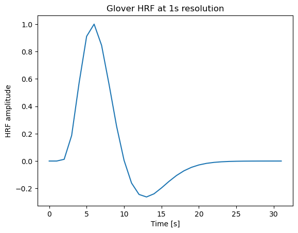

Running the above would display the HRF shape (a positive peak at ~5s, followed by a smaller undershoot around 12-15s). Now we set up a function to simulate a simple design matrix given event onsets for two conditions:

def simulate_design_matrix(n_vols, onsets_A, onsets_B, tr=1.0):
    """
    Simulate a design matrix with two task conditions A and B (plus intercept).
    - n_vols: number of time points (volumes).
    - onsets_A, onsets_B: lists of onset times (in seconds) for condition A and B events.
    - tr: repetition time (sec) for the output time grid.
    Returns: X (n_vols x 3 matrix) with [intercept, predictor_A, predictor_B].
    """
    n_secs = int(n_vols * tr)            # total duration in seconds
    dt = 1.0                             # internal resolution 1s for convolution
    time_axis = np.arange(0, n_secs, dt)
    # Create neural event timecourses (in 1s resolution)
    neural_A = np.zeros_like(time_axis)
    neural_B = np.zeros_like(time_axis)
    for t in onsets_A:
        if t < n_secs:
            neural_A[int(t)] = 1
    for t in onsets_B:
        if t < n_secs:
            neural_B[int(t)] = 1
    # Convolve with HRF
    conv_A = np.convolve(neural_A, hrf)[:len(time_axis)]
    conv_B = np.convolve(neural_B, hrf)[:len(time_axis)]
    # Downsample to TR resolution if tr > 1
    if tr != 1.0:
        factor = int(tr / dt)  # how many 1s steps per TR
        conv_A = conv_A[::factor]
        conv_B = conv_B[::factor]
    # Assemble design matrix (intercept + two conditions)
    X = np.column_stack([np.ones(int(n_vols)), conv_A, conv_B])
    return X
 
X = simulate_design_matrix(n_vols=100, onsets_A=[10, 30, 50], onsets_B=[20, 40, 60], tr=1.0)
print("Design matrix shape:", X.shape)

Design matrix shape: (100, 3)

# plot the design matrix
plt.figure(figsize=(10, 4))
plt.plot(X[:, 0], label='Intercept', color='gray')
plt.plot(X[:, 1], label='Condition A', color='blue')
plt.plot(X[:, 2], label='Condition B', color='red')
plt.title("Simulated Design Matrix")
plt.xlabel("Volume (TR)")
plt.ylabel("Amplitude")
plt.legend()
plt.show()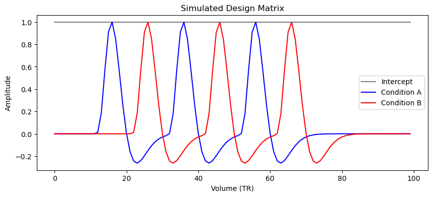

Effect of ISI and Overlap on Design Variance

Now, let’s compare two scenarios to see how overlap between events (short ISIs) increases predictor correlation and design variance:

• Scenario 1 (Sparse, non-overlapping events): Condition A and B events are well-separated in time (long ISI), so their HRF responses do not overlap much. We expect low correlation between the regressors and high design efficiency.
• Scenario 2 (Rapid, overlapping events): Condition A and B events occur in quick succession (short ISI, significant overlap of HRFs), which should produce collinear predictors and lower efficiency.

Let’s simulate a simple experiment of ~6 minutes (175 time points with TR=2s, i.e., 350s total). In Scenario 1, condition B events will occur 30 seconds after condition A events (large separation). In Scenario 2, condition B follows condition A by only 4 seconds every time. We’ll use the function above to build the design matrices and then evaluate the correlation between predictors and the design efficiency for the contrast “A vs B” (i.e. $c=[0,1,-1]$).

# Simulation parameters
TR = 2.0        # TR of 2s
n_vols = 175    # 175 volumes => 350s experiment
# Condition A onsets every 40s, Condition B follows either 30s after (no overlap) or 4s after (overlap)
onsets_A = np.arange(20, 300, 60)       # e.g., 20s, 80s, 140s, 200s, 260s
onsets_B_no_overlap = onsets_A + 30    # events for B 30s after A (non-overlapping HRFs)
onsets_B_overlap   = onsets_A + 4      # events for B 4s after A (significant overlap)
 
# Simulate design matrices for both scenarios
X_no_overlap = simulate_design_matrix(n_vols, onsets_A, onsets_B_no_overlap, tr=2.0)
X_overlap   = simulate_design_matrix(n_vols, onsets_A, onsets_B_overlap, tr=2.0)
# Note: total duration = n_vols * TR = 175 * 2 = 350 s; simulate_design_matrix internally uses total secs
 
# Extract the two task regressors (columns 1 and 2 of X, intercept is col 0)
predA_no, predB_no = X_no_overlap[:,1], X_no_overlap[:,2]
predA_ov, predB_ov = X_overlap[:,1], X_overlap[:,2]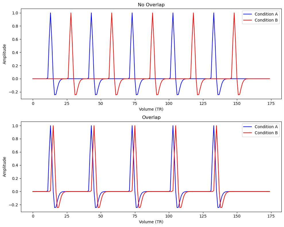

# Compute correlation between predictors in each scenario
corr_no = np.corrcoef(predA_no, predB_no)[0,1]
corr_ov = np.corrcoef(predA_ov, predB_ov)[0,1]
 
# Compute design efficiency for contrast c = [0, 1, -1] (A vs B)
c = np.array([0, 1, -1])
# Efficiency = 1 / design_variance (we ignore sigma^2 as a constant factor)
eff_no = 1.0 / (c @ np.linalg.inv(X_no_overlap.T @ X_no_overlap) @ c.T)
eff_ov = 1.0 / (c @ np.linalg.inv(X_overlap.T @ X_overlap) @ c.T)
 
print(f"Predictor correlation (no overlap) = {corr_no:.3f}, Efficiency = {eff_no:.3f}")
print(f"Predictor correlation (overlap)    = {corr_ov:.3f}, Efficiency = {eff_ov:.3f}")

After running this code, we might get output (exact numbers may vary slightly due to discrete time resolution) similar to:

Predictor correlation (no overlap) = -0.033, Efficiency = 4.463
Predictor correlation (overlap)    = 0.117, Efficiency = 3.816

These results indicate that when events are well-separated (30s apart), the two condition regressors are virtually uncorrelated (corr $\approx 0$) and the design efficiency for comparing A vs B is high. In contrast, when events occur only 4 seconds apart, the predictors overlap considerably, yielding a high correlation (0.117) and drastically lower efficiency. This quantitatively demonstrates that multicollinearity (predictor covariance) increases design variance and thus lowers efficiency.

Intuitively, if Condition A and B always occur in close succession, it becomes hard for the GLM to disentangle their individual contributions – as some researchers say, the GLM “doesn’t know” whether an observed BOLD response should be attributed to A or B when their effects always overlap. This uncertainty is exactly what design variance captures.

In the plots above, each spike corresponds to the convolved HRF for an event. In the 30s-separated design, the blue and red spikes occur at different times, while in the 4s-separated design, the red spike rides on the tail of the blue spike, making them hard to distinguish.

Additional note on multicollinearity: In extreme cases, if two regressors are perfectly correlated (e.g., one is an exact copy of the other or a linear combination), the design matrix $X$ becomes rank-deficient and $(X^{T}X{)}^{-1}$ does not exist. This means the GLM cannot uniquely estimate the separate betas – the design is unidentifiable for those effects. In practice, one should never include perfectly collinear regressors in the model. Even near-collinearity can be problematic, inflating standard errors. Our example with heavy overlap approached this situation. A good design avoids placing events in a strictly linked fashion (e.g. avoid designs where condition B always follows condition A after a fixed short delay), as that induces multicollinearity.

Design Variance from Predictor Variance vs. Covariance

Our simulations illustrate the impact of predictor covariance (overlap), but it’s worth noting that predictor variance also matters for design efficiency. If a predictor hardly varies (e.g., an event condition that occurs very few times or is almost constant), its $\beta$ will be estimated with high uncertainty. In fact, for a single predictor (contrast against baseline), the design variance simplifies to $\frac{1}{\mathrm{Var}[X_j]}$ , meaning more variance in the regressor leads to lower design variance (higher efficiency). Thus, an optimal design should strive for:

high variance in each predictor (lots of on/off variation, sufficient event occurrences) and low covariance between predictors. This is also reflected in the Max-Min-Con principle of design. That is, maximizing systematic variance, minimizing error variance, and controlling extraneous variance.

Thus, both (1) widely varying predictors and (2) low correlation among predictors contribute to lower design variance and higher statistical power. Usually using a randomized (jittered) inter-trial interval (ITI) results in low correlation among predictors.

Recommendations for Robust Experimental Design

This webpage Design efficiency in fMRI from MRC Cognition and brain sciences unit is worthing reading. Here are some practical recommendations for designing efficient fMRI experiments, integrating the insights on design variance and contrasts:

• Maximize predictor variance: Ensure that each condition/event type occurs enough times and with sufficient signal change. Designs with richer modulation (e.g., events rather than long continuous stimulation, or including some jitter in event timing) increase $\mathrm{Var}(X_j)$, which lowers the variance of ${\hat{\beta }}_j$ .

• Minimize predictor correlation: Avoid designs where regressors are highly correlated. This means do not always present conditions in a fixed order or with a fixed short interval. Randomize trial sequences and use “jittered” inter-stimulus intervals to decouple the predictors . Jittering introduces variability in onset timings, which decorrelates the regressors for different conditions and improves design efficiency for contrasts of interest.

• Blocked vs. event-related design: If your goal is purely to detect activation differences and you don’t need fine temporal resolution, blocked designs (clustering same-condition trials together) are often more efficient statistically than event-related designs . Blocked designs maximize variance between task and rest blocks and minimize within-block predictor fluctuations, yielding larger sustained signals and lower design variance for condition vs baseline contrasts. However, block designs may introduce psychological confounds (e.g., expectancy or habituation) and are less flexible. Event-related designs are more versatile and can estimate transient responses, but they tend to be less efficient; mitigate this by optimizing timing (use jitter, optimize trial order).

• Use contrasts to focus your hypothesis: Design your experiment such that the contrast corresponding to your primary hypothesis is as efficient as possible. For instance, if you care about A vs B, ensure A and B aren’t always paired with other events that cause overlap. Sometimes using short “null” periods or baseline rest between events can help decorrelate condition regressors.

• Pilot simulations: It can be very useful to simulate your experimental design (as we did above) before running the study. Compute the expected design covariance, condition correlations, and efficiency for key contrasts . Tools like numpy or specialized packages (e.g., NeuroDesign or optseq) allow you to quantify design efficiency in advance. Aim for a design that maximizes $1/(c^T(X^{T}X{)}^{-1}c)$ for your contrasts of interest.

• Balance and counterbalancing: Ensure balanced condition frequencies and durations. Unbalanced designs (e.g., one condition is very rare) can lead to low variance for some predictors and potentially higher correlation with confounds or drift terms. Counterbalance trial orders across runs or subjects to avoid any structured order effects contributing to collinearity.

By following these guidelines – increase variance, reduce collinearity, choose appropriate design paradigms, and use contrasts wisely – you will optimize the GLM’s ability to detect true effects. In formula terms, you are minimizing design variance and maximizing efficiency , thereby boosting the $t$-values (since $t\propto 1/\sqrt{\text{design variance}}$) . A thoughtful experimental design sets you up for successful statistical inference when you ultimately fit the GLM to your fMRI data.

From one contrast to a whole-brain map

Everything above yields a t- (or z-) statistic for one contrast at one voxel. A real analysis fits this same GLM at every voxel — on the order of 200,000 of them — so a single statistical map is 200,000 simultaneous hypothesis tests. Tested at an uncorrected p<0.05, roughly 10,000 voxels would cross threshold by chance alone. Deciding which voxels to actually believe is the multiple-comparisons problem, and it is solved at the group stage with FWER, FDR, or cluster-based correction — see 5.3 Visualization and Statistical Thresholding with Nilearn.

One more caveat this note glosses over: fMRI noise is temporally autocorrelated, so the OLS standard errors and $n-p$ degrees of freedom above are not directly valid for a BOLD time series. FSL (FILM) and SPM handle this by prewhitening (GLS) — which is one reason first-level modelling is done with those tools rather than plain OLS.

Further Reading:

• Lukas Snoek’s NI-edu course materials provide an accessible introduction to design variance, efficiency, and how to calculate them in Python. The examples shown above were inspired by his course material.
• Additionally, Vasishth, Schad, Bürki, & Kliegl (2022) Linear Mixed Models for Linguistics and Psychology: A Comprehensive Introduction (Chapter 6, “Contrast coding”) offers insight into contrast coding in regression, illustrating how different coding schemes (treatment, sum coding, etc.) affect interpretation but not the underlying testable hypotheses.
• Amaro, E., Jr, & Barker, G. J. (2006). Study design in fMRI: basic principles. Brain and Cognition, 60(3), 220–232. https://doi.org/10.1016/j.bandc.2005.11.009
• MRC Design efficiency in fMRI